Building your own RiskScape model

Before we start

This tutorial is aimed at new users who want to start building their own risk models in the RiskScape Platform. We expect that you:

• Have completed the Getting started guide.

• Have a basic understanding of geospatial data and risk analysis.

• Have a Platform user account and have access to the Getting Started Platform project.

• Have applications installed on your computer that allow you to open CSV and geospatial files (i.e. GeoJSON or GeoPackage).

The aim of this tutorial is to get you familiar with building a risk model using the RiskScape wizard.

➡ Actions you need to do yourself will begin with an arrow, like this paragraph.

Note

The RiskScape Platform’s Model Wizard is currently a beta feature. You can currently build, run, and save models in the RiskScape Platform. However, you cannot share wizard models with other users, or vary the input data layers as easily as you can with other RiskScape models.

Getting started

RiskScape uses projects to organize your models. For this tutorial, we will create models in the Getting Started project. Refer back to the Getting-started guide if you want to learn more about the data being used here.

➡ Make sure you are logged into the RiskScape Platform and navigate to the Getting Started project. Then, in the left hand navigation panel, click the ‘Model Wizard’ button. Alternatively, you can click this link to go directly there.

The page should initially look like this:

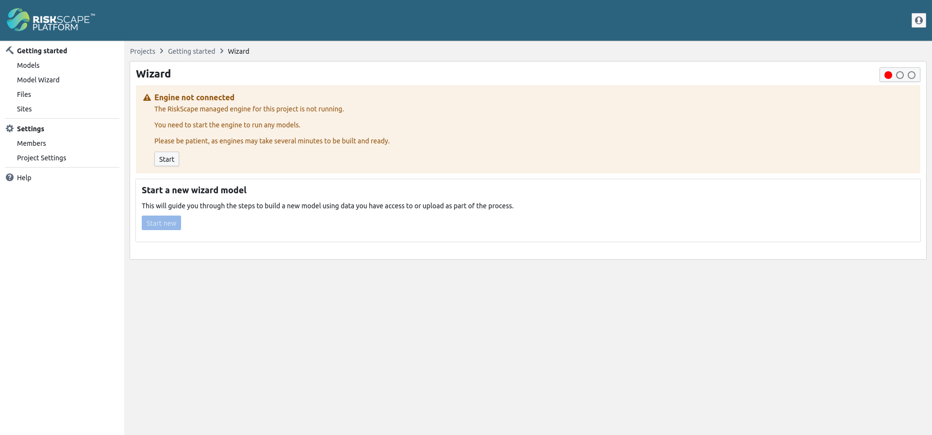
Just like the models we saw earlier in the Getting started guide, the wizard needs a RiskScape Engine in order to run.

➡ Click on the ‘Start’ button to start the Engine. It may take a while for the Engine to be created and finish starting up.

When it’s done, you’ll see a green traffic light in the upper right corner, like this:

We’re now ready to begin.

Model workflow

The processing workflow for a RiskScape model is split up into phases, which are shown in the following diagram:

graph LR subgraph Input data[Input Data] INPUT_EXPOSURES("Exposure-layer"); INPUT_HAZARD("Hazard-layer"); INPUT_AREAS("Area-layer"); end SAMPLE("Spatially<br/>Sample</>"); INPUT_EXPOSURES --> SAMPLE; INPUT_HAZARD --> SAMPLE; INPUT_AREAS --> SAMPLE; PYTHON("Python<br/>function"); SAMPLE --> ANALYSIS("Consequence<br/>Analysis"); PYTHON -.-> ANALYSIS; ANALYSIS --> REPORT("Report<br/>Results"); REPORT --> EIT("Event Impact<br/>output file"); %% Styling class INPUT_EXPOSURES,INPUT_HAZARD,PYTHON rs-box-navy class INPUT_AREAS rs-box-navy-optional class SAMPLE,ANALYSIS,REPORT rs-box class EIT rs-box-green style INPUT_AREAS color:#FFF style INPUT_EXPOSURES color:#FFF style INPUT_HAZARD color:#FFF style PYTHON color:#FFF

The grey boxes denote the model phases. The wizard will refer to these phases as Input, Sample, Analysis, and Report. We will look at each phase of the model workflow in more detail, as we go along.

The navy-coloured boxes illustrate the inputs that you provide the model with. You supply RiskScape with the input data files that the model will use, and a Python function that will analyse the impact that the hazard has on each element-at-risk.

You also need to give RiskScape instructions on how it should process the data for each phase in the model workflow. The wizard will ask you a series of questions in order to gather all the information it needs to build a model.

Creating a building damage model

To start with, we will replicate the ‘Building-damage’ model from the getting started tutorial. This model determines if a building was exposed to the tsunami inundation, then estimates the damage done to it by the tsunami. More details about how the function works can be found in the getting started tutorial.

➡ Click the ‘Start new’ button to start creating your model.

You should be presented with a list of questions like this:

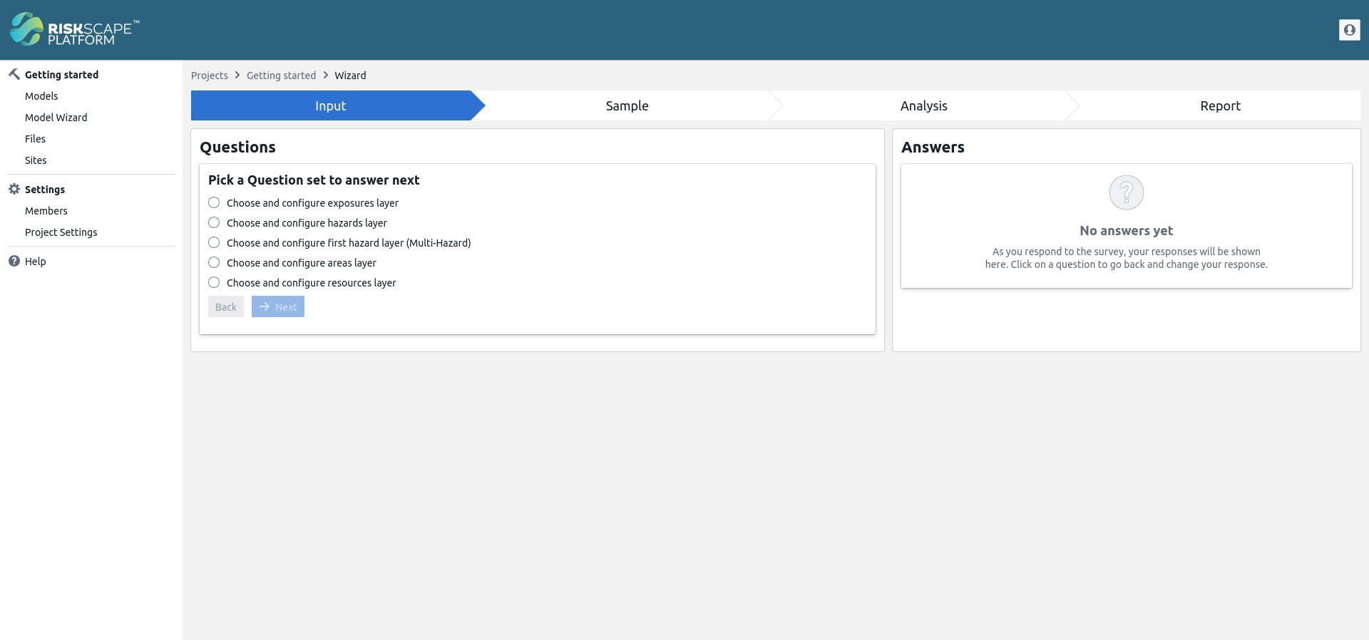
At the top of the screen, you can see the four model phases. As you complete the wizard process, this will give you a general idea of how far through you are.

The left-hand ‘Questions’ side will show you the next questions to be answered. The right-hand ‘Answers’ side will show you the previous questions you have already answered.

Let’s begin by specifying our input data.

Input phase

A RiskScape model can have the following input layers:

Exposure-layer

This contains the elements-at-risk that are potentially impacted by the hazard. For example, these could be buildings, roads, infrastructure, or even population density or land-use maps.

Hazard-layer

This contains the geospatial footprint of the hazard you are modelling.

Area-layer

This contains regional boundaries that can optionally be used to collate the results. For example, if you wanted a breakdown of damage or losses by district or region.

Resource-layer

This contains any supplementary geospatial data that may be needed by your model. For example, if you are modelling an earthquake then you may need to know the soil-type underneath a building in order to calculate liquefaction damage.

Let’s start by picking the exposure-layer for our model.

➡ Select ‘Choose and configure exposures layer’ and click ‘Next’.

The wizard will then present us with a file picker, where we can choose a data source.

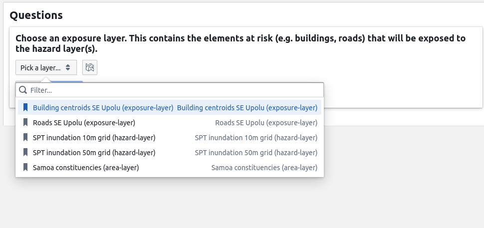
These options are the bookmarks in our project. A bookmarked data source is how we tell RiskScape about an input file to use in our model.

Note

We have already setup the getting-started project with some bookmarks, to make life easier. Bookmarks are defined in plain-text configuration files by the project owner, or administrator. Expert CLI users can learn more about how to define bookmarks here.

We want our exposure-layer to be the buildings database, so pick the first option.

➡ Click the ‘Pick a layer’ button, and select Building centroids SE Upolu (exposure-layer). Click ‘Next’.

Tip

In addition to the pre-existing bookmarks, you can also choose a file from your own computer, or from project storage. The Navigating project files tutorial will explain how file storage works in the RiskScape Platform in more detail.

The next choice the wizard presents us with looks like this:

Geoprocessing lets us manipulate the input geometry before it gets used in the model. We want to skip geoprocessing for now.

➡ Select ‘No’ for geoprocessing and click ‘Next’

RiskScape will now give you the option of specifying the other layers that your model will use:

➡ Select ‘Choose and configure hazards layer’ and click ‘Next’.
➡ Click the ‘Pick a layer’ button, and select SPT inundation 10m grid (hazard-layer). Click ‘Next’.

Note

We are not offered a follow-up geoprocessing question this time. This is because the hazard-layer is raster data (a GeoTIFF), and RiskScape only supports geoprocessing for vector data, such as shapefiles.

Undoing mistakes

Your answers will appear on the right hand side of the window. If you make a mistake when answering a question, you can use this to go back and fix it.

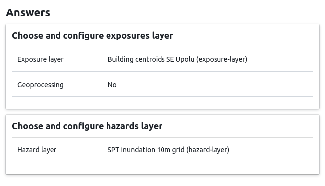
Actually, we really wanted to choose the 50m grid hazard layer here, not the 10m grid.

➡ Hover your mouse over the answer to the hazard layer question. An edit (pencil icon) button should appear to the right. Click that button.
➡ Select the drop-down, and choose ‘SPT inundation 50m grid (hazard-layer)’. Click ‘Next’.

We don’t want to add any more layers, so let’s move on to the next phase.

➡ Select ‘skip’, and click ‘Next’.

Sample phase

➡ Select ‘Sampling Phase’ and click ‘Next’.

At the top of the page, note that the ‘Sample’ phase is now coloured blue, indicating that we’ve moved into a new phase.

In the Spatial Sampling phase, RiskScape geospatially combines the input layers in your model. For example, it spatially matches each element-at-risk against the hazard-layer in order to determine the hazard intensity measure (if any) that affects it.

You could think of sampling as being like putting a pin into a map and plucking out the data at the point where it lands. In this case, we have the centroid of a building footprint, and we are plucking out the tsunami inundation depth at that point. Conceptually, it looks something like this:

The building data geometry that we are using here consists of centroid points, so we can simply choose ‘centroid’ sampling.

➡ Select ‘centroid’ and click ‘Next’

Tip

The ‘closest’ sampling is generally a good default choice for most models, as it works well for lines and polygons, as well as points. We use ‘centroid’ sampling in these examples purely for simplicity. Expert users can learn more about the RiskScape CLI Engine’s different spatial matching techniques here.

Analysis phase

The next phase of the model workflow is the Consequence Analysis phase. In this phase, RiskScape applies a Python function to every element-at-risk in your exposure-layer, using the hazard intensity measure that was determined by the sampling phase. This function will calculate the impact, or consequence, that the hazard has on each building.

➡ Select ‘Analysis Phase’ and click ‘Next’

RiskScape presents us with a list of functions we can potentially use for our model.

Note

Just like bookmarks, functions are defined in plain-text configuration files by the project owner, or administrator. We have already setup the getting-started project with these functions, to make life easier. Expert CLI users can learn more about how to define functions here.

As we’re replicating the Building-damage model, we’ll use the building damage function.

➡ Select ‘Building_Damage_State’ and click ‘Next’.

Report phase

The last phase of the model workflow is the Results Reporting phase. This phase lets us customize how the model results are saved to file. For now, we are going to skip this phase and come back to it later.

➡ Select ‘skip’ and click ‘Next’.

We have now gone through all the phases of the model workflow, so our model should be ready to run.

➡ Enter a name for your model (e.g. building damage) and click ‘Run’.

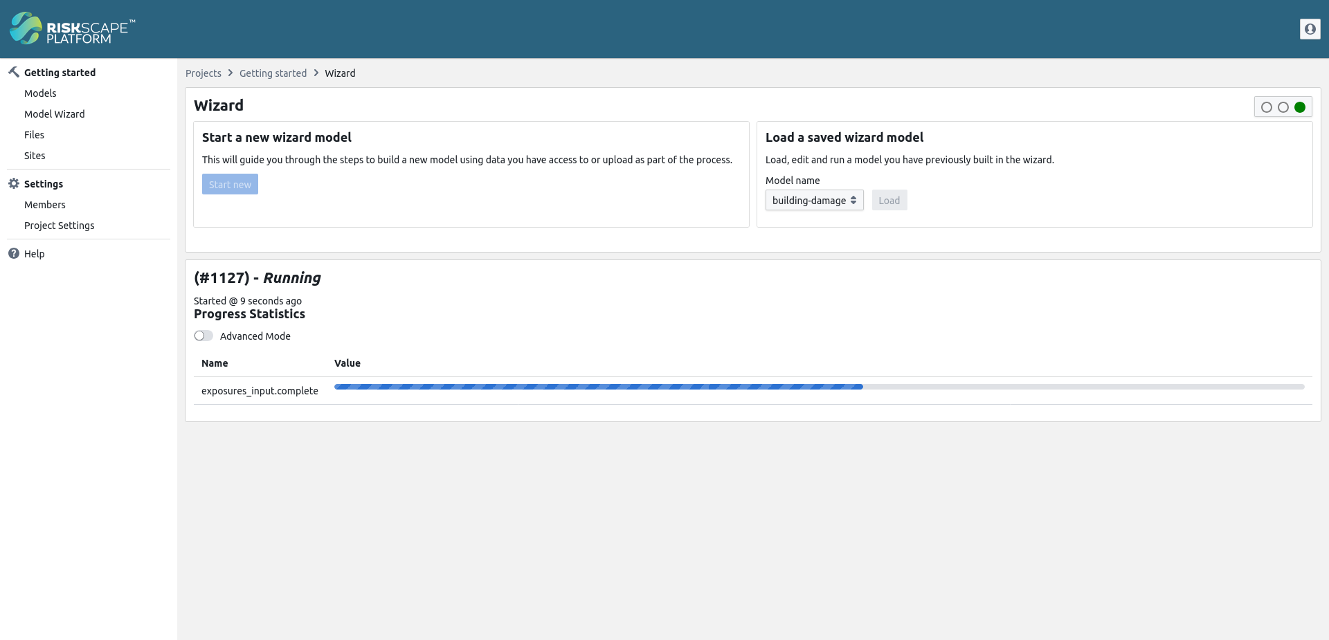
As RiskScape runs your model, you should see progress statistics displayed like the following:

➡ Once the model completes, click the ‘Download’ button for the ‘event_impact_table’ and open the file in your preferred GIS application.

Tip

If you are not comfortable using GIS software, then you may need to get a colleague to help you, or skip ahead to the next section.

The results should look similar to your previous ‘Building-damage’ model results from the getting-started tutorial. The main difference is that the building data we have used here is centroid points instead of polygon building footprints.

Note

The building damage function here uses some randomness when assigning a building damage state based on probabilities. This means that in some cases the damage state for a given building may vary between model runs.

Building a model with regional aggregation

We will now use the wizard to build a slightly more complicated model that includes an area-layer, so that we can aggregate the results by region. This means that the model results will report a total count of exposed buildings, instead of saving every single exposed building.

➡ Click ‘Start new’ to begin a new model.

Input phase

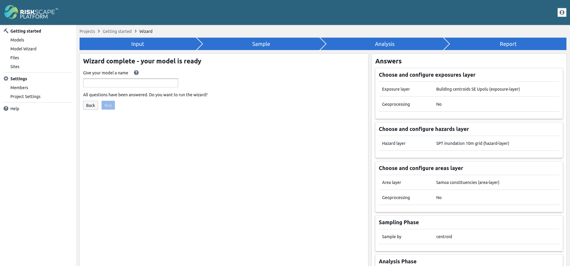
Select the same exposure-layer and hazard-layer as you did previously, i.e.

➡ Select ‘Choose and configure exposures layer’ and click ‘Next’.
➡ Click the ‘Pick a layer’ button, and select Building centroids SE Upolu (exposure-layer). Click ‘Next’.
➡ Select ‘No’ for geoprocessing and click ‘Next’
➡ Select ‘Choose and configure hazards layer’ and click ‘Next’.
➡ Click the ‘Pick a layer’ button, and select SPT inundation 10m grid (hazard-layer). Click ‘Next’.

Tip

Remember if you enter the wrong answer at any point in the wizard, you can go back and change your answer using the list of answers on the right.

This time, we will also add an area-layer to our model. In the wizard:

➡ Select ‘Choose and configure areas layer’ and click ‘Next’.
➡ Click the ‘Pick a layer’ button, and select Samoa constituencies (area-layer). Click ‘Next’.
➡ Select ‘No’ for geoprocessing and click ‘Next’
➡ Select ‘skip’, and click ‘Next’ to skip adding a resources layer

Sampling phase

Again, we will use the same sampling answers as we did in our previous model. In the wizard:

➡ Select ‘Sampling Phase’ and click ‘Next’.
➡ Select ‘centroid’ and click ‘Next’

You will now be presented with an extra optional question about the area-layer, i.e.

This ‘buffer’ option is useful when some of our elements-at-risk fall just outside the area-layer boundaries. This can be a particular problem in coastal areas, for example with ports or lighthouses that are actually located in the sea.

➡ Click ‘Skip’ to skip this option for now.

Note

When you change an answer to a wizard question, it can ‘unlock’ more follow-up questions. For example, when we specified an area-layer as input data, the wizard then presented us with an additional follow-up spatial sampling question we could answer.

Analysis phase

The is_exposed function is a built-in RiskScape function that can be used in any exposure model. The is_exposed function produces a consequence of ‘1’ if the element-at-risk was exposed to the hazard, and ‘0’ if not.

For simplicity, we’ll use the is_exposed function for this model.

➡ Select ‘is_exposed’, and click ‘Next’

Report phase

We will now look at changing how we report the results from the model.

➡ Select ‘Change how the final ‘event-impact’ results are presented and saved to file’, and click ‘Next’

There are a range of operations that RiskScape can apply to the Event Impact Table data before it is saved to file.

These are all just different ways to manipulate the results data:

• Filtering lets us exclude or include certain results, based on a given condition. For example, we could exclude ‘Outbuildings’ from the results.

• Aggregating lets us summarize or collate the results. This is similar to spreadsheet operations like COUNT() or SUM() that you would use across rows of data.

• Selecting lets us adjust or rename what attributes appear in the results file. For example, we could rename the consequence attribute to Exposed to better suit our model.

• Sorting lets you order the results. For example, we could order the results by the hazard attribute, so we can easily identify the buildings that are worst impacted by inundation.

• Finally, we can also specify the file format that the results get saved in.

➡ Click ‘Skip’ for the filter question

Aggregation

There are two parts to aggregation:

1. Grouping the results by the attribute(s) that we are interested in. This is how we want to see the model results broken down, such as by region or by building construction material.

2. Applying an aggregate function, such as sum() or count(), to each group of results. This is what collated result we want to see, such as the total count of affected buildings or the total monetary loss.

The wizard can also optionally aggregate your data into buckets, or bins. We will cover this in more detail later.

As a simple example, let’s say that our model produces a loss consequence, in dollars, and we want to see the total losses broken down by the building construction material:

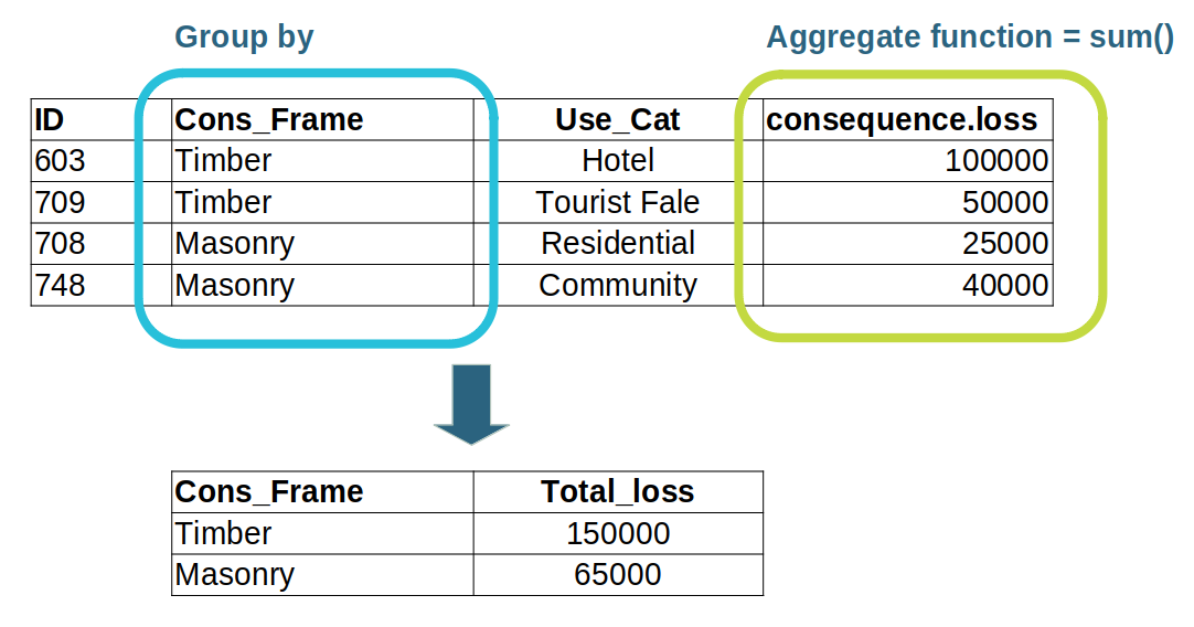
In this example, the building data is grouped based on the Cons_Frame attribute, which means buildings that share the same construction material are grouped together.

We then use the sum() aggregate function to add together the loss values for all the buildings that share the same construction material, and produce a Total_loss result.

Part 1: Group by

In the wizard, RiskScape presents us with the first choice, of how to group the results:

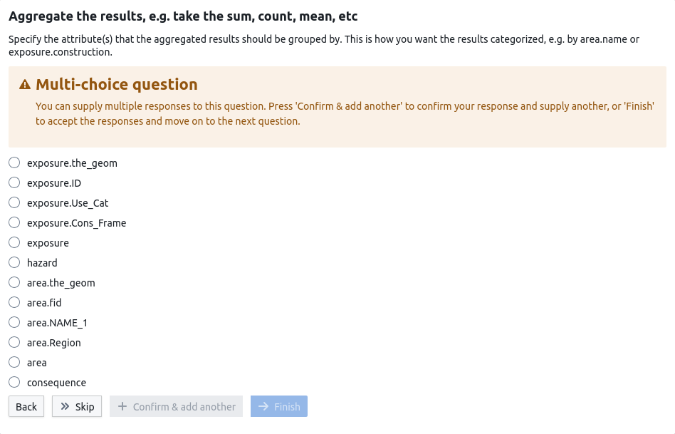
These are all the attributes that are currently in our model results.

Note

We can select either a single attribute here, or a collection of attributes. For example, area.Region is a single attribute - selecting it will aggregate by the region’s name, producing a CSV results file. Whereas area is a collection of attributes - selecting it will include the region’s name and its geometry, producing a geospatial results file.

In this case, we want to group the results by region (area.Region). This means that any rows of data that have the same region will be grouped together. In the wizard:

➡ Select ‘area.Region’ and click ‘Finish’

Part 2: Applying an aggregate function

RiskScape will then ask you what aggregation you want to apply to the grouped data:

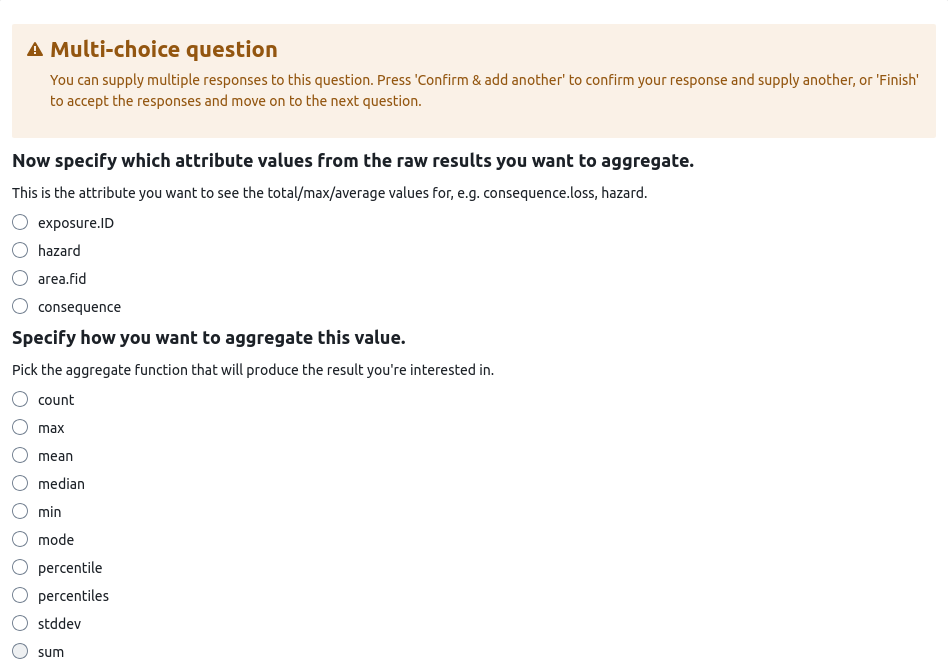
In this case we want to count the total number of buildings exposed to inundation in each region, i.e. we want to count the buildings that have a hazard value present.

➡ Select ‘hazard’ for the attribute value
➡ Select ‘count’ for how to aggregate it
➡ Enter ‘Total_exposed’ for the new name
➡ Click Finish

Tip

Using a RiskScape aggregate function is conceptually similar to using a spreadsheet formula, like SUM(A1:A20), where you have a function and a range of spreadsheet cells it applies to. Picking the attribute to aggregate is like specifying the spreadsheet column in the formula. Picking the attribute to group the data by determines which spreadsheet rows get collated together.

The wizard can also optionally aggregate your data into buckets, or bins. We will cover this in more detail later. For now, we’ll skip this.

➡ Click ‘Skip’ for the ‘Aggregate by buckets’ question
➡ Click ‘Skip’ for the ‘Select and adjust the columns’ question
➡ Select ‘Region’ and then asc for the sort question and then click ‘Finish’
➡ Click ‘Skip’ for the output file format

A RiskScape model can have multiple output files, which lets you save your results in several different ways.

➡ Select ‘skip’ and click Next
➡ Enter a new name for your model (e.g. total exposed) and click ‘Run’.

Download the ‘event-impact’ results file and open it. You will notice that the file is a CSV (spreadsheet) file, rather than a geospatial file. This is because we aggregated by region name, which is text, and so there was no geospatial data saved in the results. The results should look similar to your previous ‘Total-exposed’ model results from the getting-started tutorial.

Changing answers and re-running a model

Once you’ve run a wizard model, a new box will appear on the right hand side of the main window. This is useful if you ever want to revisit a wizard model that you previously created.

➡ Use the drop-down to select the total exposed model you created earlier, and then click ‘Load’.

The RiskScape Platform will load in your answers, just as if you’d re-entered them. Using the list on the right, you can change any of your answers.

Bucket aggregation assigns each row of data to a ‘bucket’ or ‘bin’ based on the numeric range a given value falls into, and then aggregates each bucket separately. For example, we might want to see the number of buildings exposed to different inundation depths, so that we can coordinate an emergency response effectively. In this case, we might have a few different inundation ‘bins’ (<1m, 1-2m, 2-3m, and 3m+), and we want to count the number of buildings in each bin.

Let’s change this model so that the data is aggregated by bins.

➡ Hover over your answer to the Aggregate attributes question on the right hand side (you may need to scroll down), then click the edit button.

➡ Click ‘Finish’ to move onto the bucket aggregation question.

First, the wizard will ask you how to divide the results into bins. In this case, we are interested in the inundation depth, which is the hazard attribute.

➡ Select ‘hazard’ and click ‘Next’

Next, we need to specify the boundaries for the bins. Let’s say we are interested in the depths <1m, 1-2m, 2-3m, and 3m+.

➡ Enter 1 and click ‘Confirm & add another’
➡ Enter 2 and click ‘Confirm & add another’
➡ Enter 3 and click ‘Finish’

Note

RiskScape will automatically include bins for any values that fall below the first boundary (i.e. <1m), or above the last boundary (i.e. 3m+). The remaining bins will fall between the boundaries specified (i.e. 1-2m and 2-3m).

Now we need to tell the wizard how to aggregate the data inside each bin or bucket. In this case, we want the total count of buildings exposed to each inundation depth range.

➡ Specify ‘hazard’ for the attribute value
➡ Specify ‘count’ for how to aggregate it
➡ Enter ‘Total_exposed’ for the new name
➡ Click ‘Finish’

Finally, we need to specify the name that the binned data will have in the results file.

➡ Enter a name for the aggregated data (e.g. Depth), then click ‘Next’

We now go through and finish the rest of the wizard process. Although we’re editing a saved model, we still go through all the remaining questions again, because changing one question’s answer can have flow-on effects for other questions.

➡ Click ‘Skip’ for the ‘Select and adjust the columns’ question
➡ Select ‘Region’ and then asc for the sort question and then click ‘Finish’
➡ Click ‘Skip’ for the output file format
➡ Select ‘skip’ to saving the results in a different way and click ‘Next’
➡ Enter a new name for your model (e.g. total exposed depths) and click ‘Run’.

Download and open your results file. There should now be new columns containing the binned results, e.g. Depth.range_<_1.0.Total_exposed, Depth.range_1.0_2.0.Total_exposed, Depth.range_2.0_3.0.Total_exposed, and Depth.range_3.0_+.Total_exposed.

More exercises

Here are some more exercises to try in the wizard. Do as many as you feel comfortable with.

Exposed buildings by use category

Instead of aggregating by region (area.Region), try aggregating by building use category (exposure.Use_Cat) instead. Do the following:

➡ Select the ‘total exposed’ saved wizard model and click Load
➡ Scroll down to the ‘Change how the final ‘event-impact’ results are presented and saved to file’ section
➡ Click the ‘edit’ icon for the ‘Group by…’ section
➡ Select exposure.Use_Cat and click Finish
➡ Click Finish and Skip to progress through the rest of the wizard, and run your model
➡ Download and open the results. Check how they differ to earlier wizard results.

Geospatial aggregated output

Repeat the previous exercise, but this time select area instead of area.Region or exposure.Use_Cat. This aggregates by all the area-layer’s attributes, including the geometry. You should now get a geospatial results file when you run the model. Download it and open it.

Tip

If you are using QGIS, try using feature rendering, such as the graduated rendering to identify on a map the regions that were worst affected by the tsunami.

Using different aggregation functions

➡ Select the ‘total exposed’ saved wizard model and click Load
➡ Scroll down to the ‘Change how the final ‘event-impact’ results are presented and saved to file’ section
➡ Click the ‘edit’ icon for the ‘Aggregate…’ section
➡ Select ‘hazard’, but instead of using the ‘count’ aggregate function, select ‘median’. Call the aggregated result ‘Median_Depth’, and click ‘Confirm and add another’.
➡ Repeat the process to add another aggregated value, but select the 75th percentile this time.
➡ Click Finish and Skip to progress through the rest of the wizard, and run your model
➡ Download and open the results. Check how they differ to earlier wizard results.

Looking at your model results, which three regions do you think were worst impacted by the tsunami?

Roads exposure-layer

➡ Start a new model, but select the Roads SE Upolu (exposure-layer) input instead of the buildings layer.
➡ Use the 10m hazard-layer with no area-layer
➡ Use ‘closest’ sampling, and skip the buffer distance.
➡ Use the is_exposed analysis function
➡ Skip the remaining questions and run the model
➡ Download the results and open them in your preferred GIS application

Tip

With large exposure-layer features, such as roads, you would typically cut the roads into smaller pieces (e.g. 10m segments). RiskScape’s geoprocessing features let you do this in the model-building wizard.

Try downloading the hazard-layer and viewing it alongside your road model results in your GIS application.